The Unification of DDPM and Score-based Models
This post explores the unification of DDPM and Score-based Models in diffusion generative modeling. We show how x-prediction and score-prediction are fundamentally equivalent, and how both can be viewed through the lens of Stochastic Differential Equations (SDEs).
DDPM from a Score Perspective
In DDPM
According to Tweedie’s Formula, we can obtain:
\[\sqrt{\bar{\alpha}_t} \boldsymbol{x}_0 = \boldsymbol{x}_t + (1 - \bar{\alpha}_t) \nabla_{x_t} \log p(\boldsymbol{x}_t) \tag{2}\]Tweedie’s Formula:
For a Gaussian variable $z\sim \mathcal N(z;\mu_z,\Sigma_z)$, we have
\[\mu_z=z+\Sigma_z\nabla_z\log p(z)\]
Meanwhile, from (1) we know
\[x_t=\sqrt{\bar{\alpha}_t}x_0+\sqrt{1-\bar{\alpha}_t}\epsilon_t\]Substituting into (2), we obtain
\[\nabla_{x_t}\log p(x_t)=-\frac{\epsilon_t}{\sqrt{1-\bar{\alpha}_t}}\]Thus
\[\begin{align*} \boldsymbol{\mu}_q &= \frac{1}{\sqrt{\alpha_t}} \boldsymbol{x}_t - \frac{1 - \alpha_t}{\sqrt{1 - \bar{\alpha}_t} \sqrt{\alpha_t}} \boldsymbol{\varepsilon}_t\\ &=\frac{1}{\sqrt{\alpha_t}} \boldsymbol{x}_t + \frac{1 - \alpha_t}{\sqrt{\alpha_t}} \color{red}\nabla_{x_t} \log p(\boldsymbol{x}_t) \end{align*}\]Similarly, we model the reverse process as
\[\begin{align*} \boldsymbol{\mu}_{\theta} &= \frac{1}{\sqrt{\alpha_t}} \boldsymbol{x}_t - \frac{1 - \alpha_t}{\sqrt{1 - \bar{\alpha}_t} \sqrt{\alpha_t}} \boldsymbol{\varepsilon}_{\theta}(x_t,t)\\ &=\frac{1}{\sqrt{\alpha_t}} \boldsymbol{x}_t + \frac{1 - \alpha_t}{\sqrt{\alpha_t}} \color{red}s_{\theta}(x_t,t) \end{align*}\]Therefore, we transform the estimation of $\epsilon_t$ and $\epsilon_{\theta}$ in DDPM into the estimation of $\nabla\log p(x)$, which gives
\[\begin{align*} &\arg\min_{\theta} D_{\text{KL}} \left( q(\boldsymbol{x}_{t-1} \vert \boldsymbol{x}_t, \boldsymbol{x}_0) \parallel p_{\theta}(\boldsymbol{x}_{t-1} \vert \boldsymbol{x}_t) \right) \\ =& \arg\min_{\theta} \frac{1}{2\sigma_q^2(t)} \left[ \lVert \boldsymbol{\mu}_{\theta} - \boldsymbol{\mu}_q \rVert_2^2 \right] \\ =& \arg\min_{\theta} \frac{1}{2\sigma_q^2(t)} \left[ \left\lVert \frac{1 - \alpha_t}{\sqrt{\alpha_t}} s_{\theta}(\boldsymbol{x}_t, t) - \frac{1 - \alpha_t}{\sqrt{\alpha_t}} \nabla \log p(\boldsymbol{x}_t) \right\rVert_2^2 \right] \\ =& \arg\min_{\theta} \frac{1}{2\sigma_q^2(t)} \frac{(1 - \alpha_t)^2}{\alpha_t} \left[ \color{red}\lVert s_{\theta}(\boldsymbol{x}_t, t) - \nabla \log p(\boldsymbol{x}_t) \rVert_2^2 \color{black}\right] \end{align*}\]Hence, we find that the optimization objective of DDPM is actually consistent with Score-Based Models, both estimating the score function.
We further compare the optimization objective of DDPM:
\[L_t = \mathbb{E} \left[ \frac{(1 - \alpha_t)^2}{2\alpha_t (1 - \bar{\alpha}_t) \sigma^2} \color{red}\left\| \boldsymbol{\epsilon}_t - \boldsymbol{\epsilon}_\theta \left( x_t, t \right) \right\|_2^2 \color{black}\right]\]We note that when $L_t$ reaches its optimum, we have
\[\epsilon_{\theta}(x_t,t)=\mathbb E\big[\epsilon_t|x_t,t\big]=\mathbb E\big[\epsilon_t|x_0,t\big]\]This indicates that the model actually learns the mean of the noise given data $x_0$. In other words, the conditional expectation learned by our network already contains information about the true sample $x_0$, which is what enables us to obtain the distribution of true data by learning the noise.
Meanwhile, we find that under optimal conditions, $L_t$ cannot reach 0, meaning that our optimization objective does not achieve maximum likelihood between the predicted distribution and the true distribution (otherwise the loss should reduce to 0). Combined with Score-Based Models, we know this is because we are actually predicting the score of the data distribution, and there is still a certain gap between the score distribution and the data distribution.
SDE Model
What happens if we extend the finite steps $T$ to infinite steps? Experimental validation shows that larger $T$ can yield more accurate likelihood estimates and better quality results. Thus, continuous-time perturbation of data can be modeled as a stochastic differential equation (SDE).

Definition
There are many forms of SDEs. One form given by Dr. Yang Song in his paper )t and current value x) is:
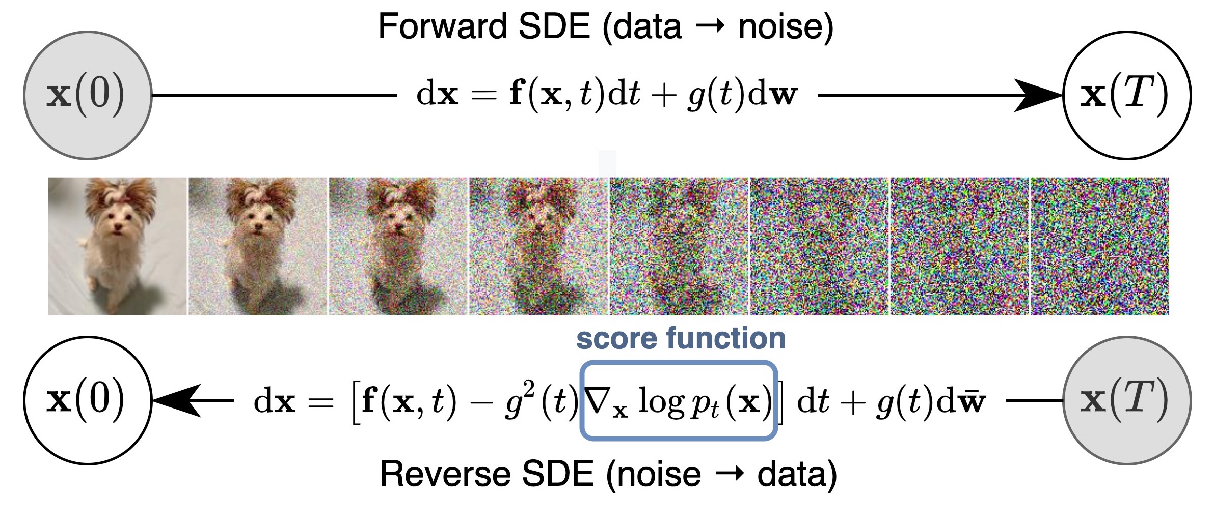
where $f(\cdot)$ is called the drift coefficient, $g(t)$ is called the diffusion coefficient, $\boldsymbol{w}$ is a standard Brownian motion, and $\mathrm{d}\boldsymbol{w}$ can be viewed as white noise. The solution to this stochastic differential equation is a set of continuous random variables $\lbrace\boldsymbol x(t)\rbrace_{t\in [0,T]}$, where $t$ represents the continuous version of the discrete form $(1, 2, \ldots, T)$.
We use $p_t(\boldsymbol{x})$ to denote the probability density function of $\boldsymbol{x}(t)$, which corresponds to the previous $p_{\sigma_t}(\boldsymbol{x}_t)$. Here $p_0(\boldsymbol{x}) = p(\boldsymbol{x})$ is the original data distribution, and $p_T(\boldsymbol{x}) = \mathcal{N}(0, \mathbf{I})$ is the white noise obtained after noise perturbation.
Brownian Motion
If a stochastic process $\lbrace X(t), t \geq 0\rbrace$ satisfies:
- $X(t)$ is an independent increment process;
- $\forall s, t > 0, X(s + t) - X(s) \sim N(0, c^2 t)$
then the stochastic process $\lbrace X(t), t \geq 0\rbrace$ is called Brownian motion (denoted as $B(t)$) or Wiener process (denoted as $W(t)$). In this text, we will subsequently denote it as $W(t)$. If $c = 1$, it is called standard Brownian motion, satisfying $W(t) \sim N(0, t)$.
Forward SDE
We can directly discretize the equation
\[\mathrm{d}\boldsymbol{x} = f(\boldsymbol{x}, t)\mathrm{d}t + g(t)\mathrm{d}\boldsymbol{w}\]where
\[\begin{aligned} dx &\to x_{t+\Delta t}-x_t\\ dt &\to \Delta t\\ dw &\to w(t+\Delta t)-w(t)\sim\mathcal N(0,\Delta t)=\sqrt{\Delta t}\epsilon \end{aligned}\]Thus, the discrete form of the SDE is represented as:
\[\color{red} x_{t+\Delta t}-x_t=f(x,t)\Delta t+g(t)\sqrt{\Delta t}\epsilon\]where $\epsilon\sim\mathcal N(0,1)$.
VE-SDE
For NCSN, the forward process (adding noise) is shown as follows:
\[\begin{aligned} x_t &= x_0+\sigma_t\epsilon\\ x_{t+\Delta t} &= x_t+\underbrace{\sqrt{\sigma_{t+\Delta t}^2-\sigma_t^2}}_{\color{red}\sqrt{\frac{\sigma_{t+\Delta t}^2-\sigma_t^2}{\Delta t}}\sqrt{\Delta t}}\epsilon \end{aligned}\]Therefore, in the corresponding SDE representation
\[\begin{aligned} f(x_t,t) &= 0\\ g(t) &= \lim\limits_{\Delta\to 0}\sqrt{\frac{\sigma_{t+\Delta t}^2-\sigma_t^2}{\Delta t}}=\sqrt{2\sigma_t\dot\sigma_t} \end{aligned}\]The corresponding continuous SDE for the VE process is:
\[\color{blue}dx=\sqrt{2\sigma_t\dot\sigma_t}dW\]VP-SDE
For DDPM, its forward process is represented as follows:
\[\begin{aligned} x_t &= \sqrt{\bar{\alpha}_t}x_0+\sqrt{1-\bar{\alpha}_t}\epsilon\\ x_{t+1} &= \sqrt{1-\beta_{t+1}}x_t+\sqrt{\beta_{t+1}}\epsilon \end{aligned}\]We continualize the discrete time $1,2,\cdots,t,\cdots T$ to $[0,1]$, i.e., let
\[\begin{aligned} t &\to\frac{t}{T}=t'\\ 1 &\to\frac{1}{T}=\Delta t \end{aligned}\]We can also let $\beta_{t’}=T\beta_t$, thus
\[\begin{align*} x_{t'+\Delta t}&=x_{t+1}=\sqrt{1-\beta_{t+1}}x_t+\sqrt{\beta_{t+1}}\epsilon\\ &=\sqrt{1-\beta_{t'+\Delta t}\Delta t}\cdot x_{t'}+\sqrt{\beta_{t'+\Delta t}\Delta t}\cdot \epsilon\\ &=\big(1-\frac{1}{2}\beta_{t'}\Delta t\big)x_{t'}+\sqrt{\beta_{t'}}\sqrt{\Delta t}\epsilon \end{align*}\]Therefore, in the corresponding SDE representation, we have
\[\begin{aligned} f(x_t,t) &= -\frac{1}{2}\beta_{t'}x_t\\ g(t) &= \sqrt{\beta_{t'}} \end{aligned}\]The corresponding continuous SDE for the VP process is:
\[\color{blue}dx=-\frac{1}{2}\beta_{t'}x_tdt+\sqrt{\beta_{t'}}dW\]We expect that when $t\to T$, the image becomes pure noise, then $\sigma_t\to\infty$, but $\bar{\alpha}_t\to 0$ is sufficient. This requires that in NCSN, the variance of noise gradually expands, while in DDPM, the noise variance remains between $(0,1)$. Therefore, they are respectively called VE-SDE and VP-SDE.
Reverse SDE
Using the discrete forward SDE, we can derive its reverse process. From the forward SDE:
\[\color{red} x_{t+\Delta t}-x_t=f(x,t)\Delta t+g(t)\sqrt{\Delta t}\epsilon\]we have the conditional probability:
\[x_{t+\Delta t}|x_t\sim \mathcal{N}(x_t+f(x_t,t)\Delta t, g^2(t)\Delta tI)\]Considering the reverse process from $x_{t+\Delta t}$ to $x_t$, we have the conditional probability:
\[\begin{align*} p(x_t|x_{t+\Delta t})&=\frac{p(x_{t+\Delta t}|x_t)p(x_t)}{p(x_{t+\Delta t})}\\ &=p(x_{t+\Delta t}|x_t)\exp(\log p(x_t)-\log p(x_{t+\Delta t}))\\ &\approx p(x_{t+\Delta t}|x_t)\exp\{\color{red} -(x_{t+\Delta t}-x_t)\nabla_{x_t}\log p(x_t)-\Delta t\frac{\partial}{\partial t}\log p(x_t) \color{black}\}\\ &\propto \exp\{ -\frac{\|x_{t+\Delta t}-x_t-f(x_t,t)\Delta t\|_2^2}{2g^2(t)\Delta t} - (x_{t+\Delta t}-x_t)\nabla_{x_t}\log p(x_t)-\Delta t\frac{\partial}{\partial t}\log p(x_t) \}\\ &=\exp\bigg\{ -\frac{1}{2g^2(t)\Delta t}\|(x_{t+\Delta t}-x_t)-\big[f(x_t,t)-g^2(t)\nabla_{x_t}\log p(x_t) \big]\Delta t\|_2^2 - \Delta t\frac{\partial}{\partial t}\log p(x_t)-\frac{f^2(x_t,t)\Delta t}{2g^2(t)}+\frac{\|f(x_t,t)-g^2(t)\nabla_{x_t}\log p(x_t) \|_2^2\Delta t}{2g^2(t)} \bigg\}\\ &\stackrel{\Delta t \to 0}{=} \exp\bigg\{ -\frac{1}{2g^2(t)\Delta t}\| (x_{t+\Delta t}-x_t)-\big[f(x_t,t)-g^2(t)\nabla_{x_t}\log p(x_t) \big]\Delta t \|_2^2 \bigg\} \end{align*}\]Therefore, $x_t|x_{t+\Delta t}$ follows a Gaussian distribution with mean and variance as follows:
\[\begin{aligned} \mu &= x_{t+\Delta t}-\big[f(x_t,t)-g^2(t)\nabla_{x_t}\log p(x_t) \big]\Delta t\\ \sigma^2 &= g^2(t)\Delta t \end{aligned}\]Thus, we can obtain both the discrete and continuous forms of the reverse SDE process:
\[x_{t+\Delta t}-x_t=\big[f(x_t+\Delta t,t+\Delta t)-g^2(t+\Delta t)\nabla_{x_t+\Delta t}\log p(x_{t+\Delta t}) \big]\Delta t+g(t+\Delta t)\sqrt{\Delta t}\epsilon\] \[\color{blue}dx=\big[f(x_t,t)-g^2(t)\color{red}\nabla_{x_t}\log p(x_t)\color{blue} \big]dt+g(t)dW\]
Therefore, after we have learned the score function, the reverse process becomes completely solvable. During generation, we start by sampling $x_T \sim \mathcal{N}(0, 1)$, and gradually obtain $x_0$ using the discrete process above. This discretization method for stochastic differential equations is also called the Euler–Maruyama method.
For NCSN, its forward VE process continuous SDE is:
\[\color{blue}dx=\sqrt{2\sigma_t\dot\sigma_t}dW\]Then its reverse process is:
\[dx=-2\sigma_t\dot\sigma_t\nabla_{x_t}\log p(x_t)dt+\sqrt{2\sigma_t\dot\sigma_t}dW\]Written in discrete form, it becomes
\[x_t-x_{t-1}=-2\sigma_t\dot\sigma_t\nabla_{x_t}\log p(x_t)\Delta t+\sqrt{2\sigma_t\dot\sigma_t}\sqrt{\Delta t}\epsilon_t\]In the case where $\sigma_t\dot\sigma_t=1$, if we set $\Delta t=\delta$ (this is done only for formal consistency, without real meaning), then we have
\[x_{t-1}=x_t+2\delta\nabla_{x_t}\log p(x_t)+\sqrt{2\delta}\epsilon\]This also unifies with the Langevin Equation mentioned earlier.
Optimization Target
Solving the reverse SDE requires us to know the terminal distribution $p_T(\boldsymbol{x})$ and the score function $\nabla_{\boldsymbol{x}} \log p_t(\boldsymbol{x})$. By design, the former is close to the prior distribution $\pi(\boldsymbol{x})$, which is fully tractable.
To estimate $\nabla_{\boldsymbol{x}} \log p_t(\boldsymbol{x})$, we train a time-dependent score-based model $s_\theta(\boldsymbol{x}, t)$ such that $s_\theta(\boldsymbol{x}, t) \approx \nabla_{\boldsymbol{x}} \log p_t(\boldsymbol{x})$. This is similar to NCSN’s $s_\theta(\boldsymbol{x}, i)$, which after training satisfies $s_\theta(\boldsymbol{x}, i) \approx \nabla_{\boldsymbol{x}} \log p_{\sigma_i}(\boldsymbol{x})$.
Our training objective for $s_\theta(\boldsymbol{x}, t)$ is a continuous weighted combination of Fisher divergences, given by
Relationship with Likelihood
When $\lambda(t)=g^2(t)$, under some regularity conditions, there exists an important connection between our weighted combination of Fisher divergences and the KL divergence from $p_0$ to $p_\theta$:
\[\begin{align*} \mathrm{KL}(p_0(\mathbf{x}) \| p_\theta(\mathbf{x})) &\leq \frac{T}{2} \mathbb{E}_{t \in \mathcal{U}(0,T)} \mathbb{E}_{p_t(\mathbf{x})} \left[ \lambda(t) \| \nabla_{\mathbf{x}} \log p_t(\mathbf{x}) - \mathbf{s}_\theta(\mathbf{x}, t) \|_2^2 \right] \\ &+ \mathrm{KL}(p_T \| \pi) \end{align*}\]Due to this special connection with KL divergence, and the equivalence between minimizing KL divergence and maximizing likelihood in model training, we call $\lambda(t)=g(t)^2$ the likelihood weighting function. Using this likelihood weighting function, we can train score-based generative models to achieve very high likelihoods.
PC Sampling
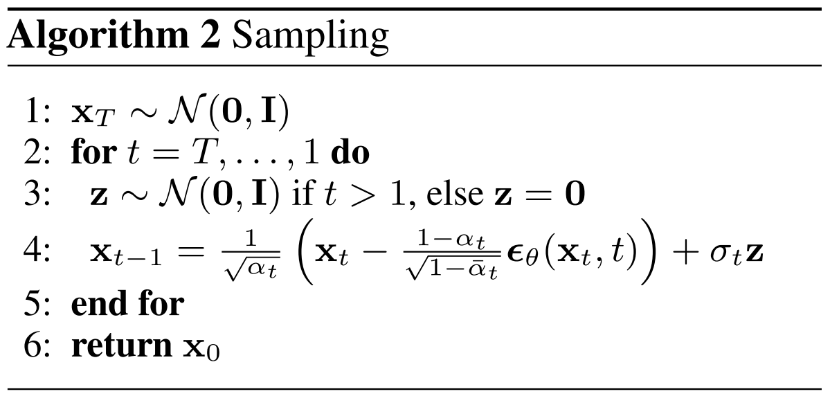
Reviewing DDPM and NCSN from an algorithmic implementation perspective, DDPM is based on the Markov assumption, assuming that samples at different times follow conditional probability distributions. Therefore, DDPM uses Ancestral Sampling to solve the SDE equation, with the algorithm shown below:

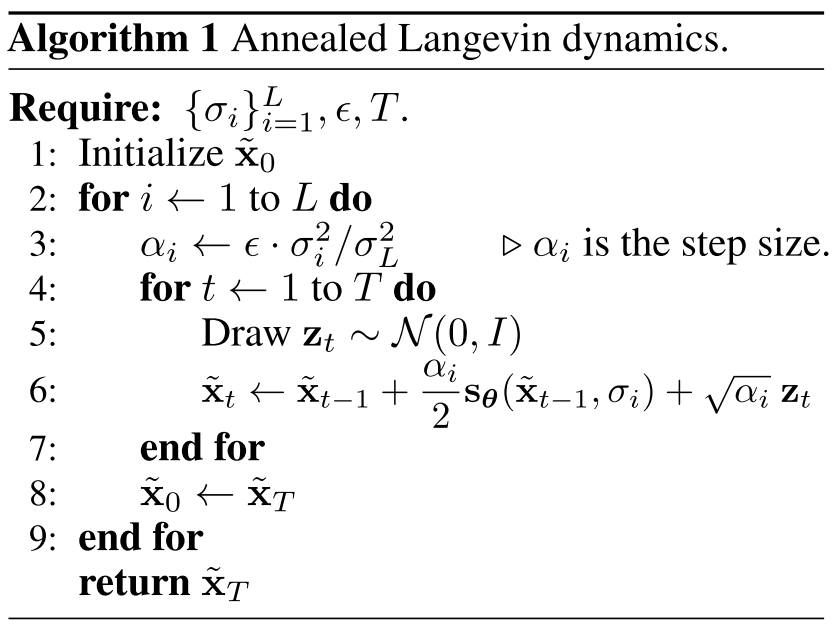
While NCSN relies on Langevin Dynamics for iterative optimization under the same noise distribution. For different noise magnitudes, there is no dependency relationship between the obtained samples. Its sampling method is shown as follows:

The former can be seen as solving the discrete form of the SDE equation, called the Predictor, while the latter can be seen as a further optimization process, called the Corrector. The author combines these two parts to present the Predictor-Corrector Sampling Method:

Probability Flow ODE
We can transform any SDE into an ODE without changing the marginal distributions $\lbrace p_t(x)\rbrace_{t\in[0,T]}$ of the stochastic differential equation. Therefore, by solving this ODE, we can sample from the same distribution as the Reverse SDE. The ODE corresponding to the SDE is called the Probability flow ODE, with the form:
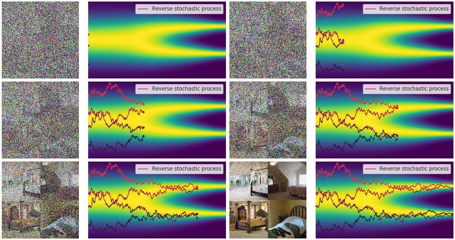
\[\color{blue}dx=\big[f(x_t,t)-\frac{1}{2}g^2(t)\color{red}\nabla_{x_t}\log p(x_t)\color{blue} \big]dt\]The figure below depicts trajectories of stochastic differential equations (SDEs) and probability flow ordinary differential equations (ODEs). It can be seen that ODE trajectories are significantly smoother than SDE trajectories, and they transform the same data distribution into the same prior distribution and vice versa, sharing the same set of marginal distributions $\lbrace p_t(\boldsymbol{x})\rbrace_{t\in[0,T]}$. In other words, trajectories obtained by solving the probability flow ODE have the same marginal distributions as SDE trajectories.

Using probability flow ODEs provides many benefits:
- Exact likelihood computation
- Manipulating latent representations
- Uniquely identifiable encoding
- Efficient sampling
Conditional Generation
According to Bayes’ theorem
\[p(x|y)=\frac{p(x)p(y|x)}{p(y)}\]Taking the score with respect to $x$ on both sides gives
\[\nabla_x\log p(x|y)=\nabla_x\log p(x)+\nabla_x\log p(y|x)\]Both latter terms are score functions that we can estimate. Therefore, we can generate $p(x|y)$ by solving the reverse SDE.
Enjoy Reading This Article?
Here are some more articles you might like to read next: